傅里叶变换
傅里叶级数
傅里叶级数:任何周期函数都可表示为不同频率的正弦函数和或余弦函数和,其中每个正弦函数和或余弦函数和都有不同的系数。
f ( t ) = ∑ n = − ∞ ∞ c n e j 2 π n T t f(t)=\sum_{n=-\infty}^\infty c_ne^{j\frac {2\pi n} {T}t}
f ( t ) = n = − ∞ ∑ ∞ c n e j T 2 π n t
其中,
c n = 1 T ∫ − T / 2 T / 2 f ( t ) e − j 2 π n T t d t , n = 0 , ± 1 , ± 2 , … c_n=\frac 1T\int_{-T/2}^{T/2}f(t)e^{-j\frac {2\pi n} {T}t}dt,n=0,\pm 1,\pm 2,…
c n = T 1 ∫ − T / 2 T / 2 f ( t ) e − j T 2 π n t d t , n = 0 , ± 1 , ± 2 , …
是系数。此篇j表示虚数单位: j 2 = − 1 j^2=-1 j 2 = − 1
傅里叶变换
傅里叶变换:(曲线下方面积有限的)非周期函数也能用正弦函数和/或余弦函数乘以加权函数的积分来表示
这表明用傅里叶级数或变换表示的函数可由逆过程完全重建(复原),而不丢失信息;允许我们工作在傅里叶域,然后返回到函数的原始域中,而不会丢失任何信息。
计算机慢慢出现了快速傅里叶变换算法(FFT),使用FFT进行频率域处理比不可分离核的空间域处理要快。
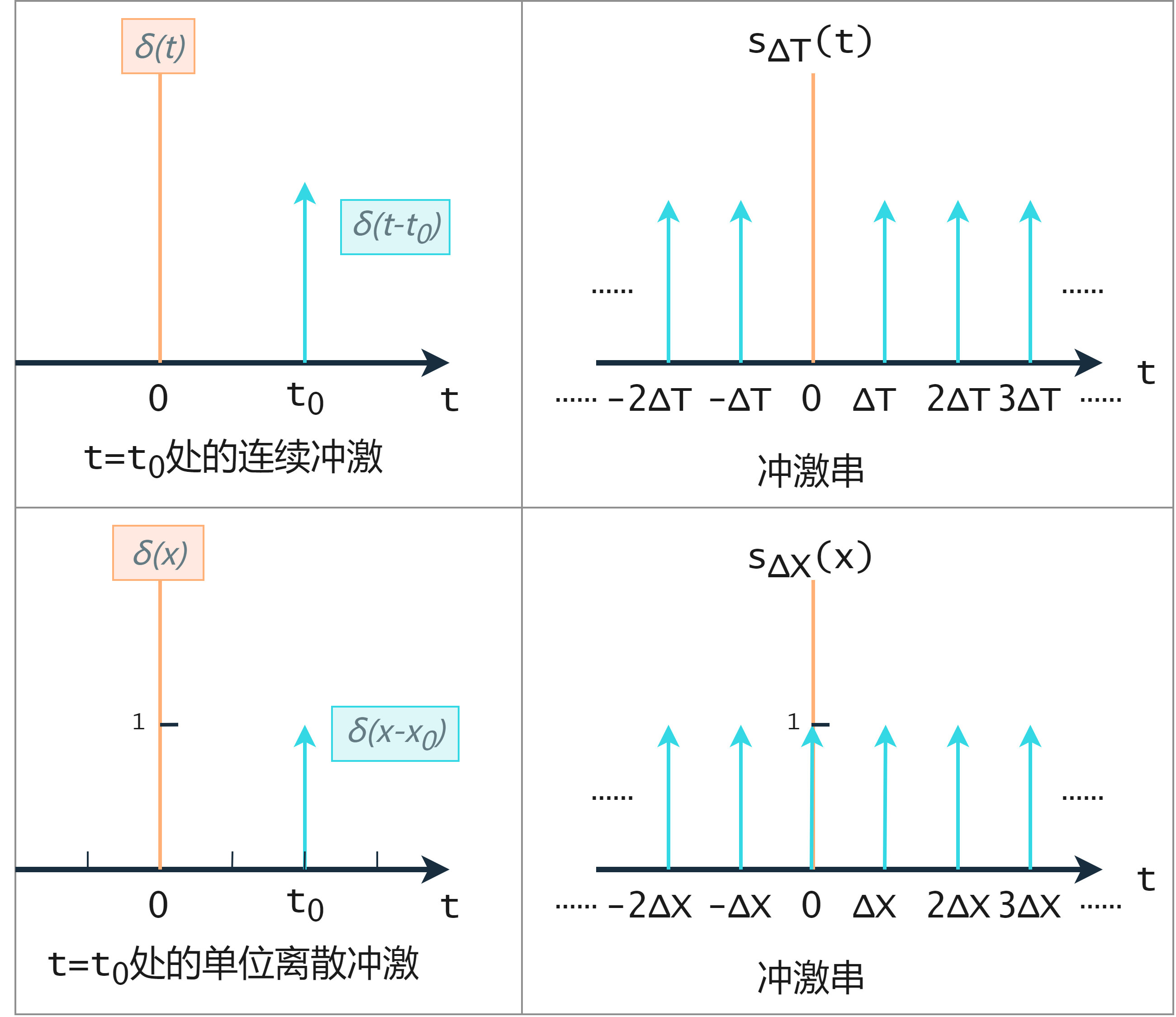
冲激函数及其取样(筛选)性质
连续变量t在t=0处的单位冲激表示为 δ ( t ) \delta(t) δ ( t )
δ ( t ) = { ∞ , t = 0 0 , t ≠ 0 \delta(t)=\begin{cases}
\infty,&t=0\\
0, &t\neq 0
\end{cases}
δ ( t ) = { ∞ , 0 , t = 0 t = 0
该定义被限制满足:
∫ − ∞ ∞ δ ( t ) d t = 1 \int_{-\infty}^{\infty}\delta(t)dt=1
∫ − ∞ ∞ δ ( t ) d t = 1
当t解释为时间时,冲激可视作幅度为无线、持续时间为0、具有单位面积的尖峰信号。
冲激具有关于积分的所谓 取样性质 :
∫ − ∞ ∞ f ( t ) δ ( t ) d t = f ( 0 ) \int_{-\infty}^{\infty}f(t)\delta(t)dt=f(0)
∫ − ∞ ∞ f ( t ) δ ( t ) d t = f ( 0 )
对其一般化,任意一点 t 0 t_0 t 0 δ ( t − t 0 ) \delta(t-t_0) δ ( t − t 0 )
∫ − ∞ ∞ f ( t ) δ ( t − t 0 ) d t = f ( t 0 ) \int_{-\infty}^{\infty}f(t)\delta(t-t_0)dt=f(t_0)
∫ − ∞ ∞ f ( t ) δ ( t − t 0 ) d t = f ( t 0 )
举一个小例子,取 f ( t ) = cos ( t ) f(t)=\cos(t) f ( t ) = cos ( t ) δ ( t − π ) \delta(t-\pi) δ ( t − π ) f ( π ) = cos ( π ) = − 1 f(\pi)=\cos(\pi)=-1 f ( π ) = cos ( π ) = − 1
冲激串则是无穷多个冲激 Δ T \Delta T Δ T
s Δ T ( t ) = ∑ k = − ∞ ∞ δ ( t − k Δ T ) s_{\Delta T}(t)=\sum_{k=-\infty}^{\infty}\delta(t-k\Delta T)
s Δ T ( t ) = k = − ∞ ∑ ∞ δ ( t − k Δ T )
单位离散冲激 δ ( x ) \delta(x) δ ( x ) δ ( t ) \delta(t) δ ( t )
δ ( x ) = { 1 , x = 0 0 , x ≠ 0 \delta(x)=\begin{cases}
1,&x=0\\
0, &x\neq 0
\end{cases}
δ ( x ) = { 1 , 0 , x = 0 x = 0
该定义被限制的离散等效形式为:
∑ x = − ∞ ∞ δ ( x ) = 1 \sum_{x=-\infty}^{\infty}\delta(x) = 1
x = − ∞ ∑ ∞ δ ( x ) = 1
离散变量的取样性质的形式为:
∑ x = − ∞ ∞ f ( x ) δ ( x ) = f ( 0 ) \sum_{x=-\infty}^{\infty}f(x)\delta(x)=f(0)
x = − ∞ ∑ ∞ f ( x ) δ ( x ) = f ( 0 )
一般式为:
∑ x = − ∞ ∞ f ( x ) δ ( x − x 0 ) = f ( x 0 ) \sum_{x=-\infty}^{\infty}f(x)\delta(x-x_0)=f(x_0)
x = − ∞ ∑ ∞ f ( x ) δ ( x − x 0 ) = f ( x 0 )
小结:
项
连续变量t
离散变量x
在0处的单位冲激
δ ( t ) = { ∞ , t = 0 0 , t ≠ 0 \delta(t)=\begin{cases}\infty,&t=0\\0, &t\neq 0\end{cases} δ ( t ) = { ∞ , 0 , t = 0 t = 0 δ ( x ) = { 1 , x = 0 0 , x ≠ 0 \delta(x)=\begin{cases}1,&x=0\\0, &x\neq 0\end{cases} δ ( x ) = { 1 , 0 , x = 0 x = 0
单位冲激满足
∫ − ∞ ∞ δ ( t ) d t = 1 \int_{-\infty}^{\infty}\delta(t)dt=1 ∫ − ∞ ∞ δ ( t ) d t = 1 ∑ x = − ∞ ∞ δ ( x ) = 1 \sum_{x=-\infty}^{\infty}\delta(x) = 1 ∑ x = − ∞ ∞ δ ( x ) = 1
取样性质
∫ − ∞ ∞ f ( t ) δ ( t ) d t = f ( 0 ) \int_{-\infty}^{\infty}f(t)\delta(t)dt=f(0) ∫ − ∞ ∞ f ( t ) δ ( t ) d t = f ( 0 ) ∑ x = − ∞ ∞ f ( x ) δ ( x ) = f ( 0 ) \sum_{x=-\infty}^{\infty}f(x)\delta(x)=f(0) ∑ x = − ∞ ∞ f ( x ) δ ( x ) = f ( 0 )
取样性质一般化
∫ − ∞ ∞ f ( t ) δ ( t − t 0 ) d t = f ( t 0 ) \int_{-\infty}^{\infty}f(t)\delta(t-t_0)dt=f(t_0) ∫ − ∞ ∞ f ( t ) δ ( t − t 0 ) d t = f ( t 0 ) ∑ x = − ∞ ∞ f ( x ) δ ( x − x 0 ) = f ( x 0 ) \sum_{x=-\infty}^{\infty}f(x)\delta(x-x_0)=f(x_0) ∑ x = − ∞ ∞ f ( x ) δ ( x − x 0 ) = f ( x 0 )
冲激串:
s Δ T ( t ) = ∑ k = − ∞ ∞ δ ( t − k Δ T ) s_{\Delta T}(t)=\sum_{k=-\infty}^{\infty}\delta(t-k\Delta T)
s Δ T ( t ) = k = − ∞ ∑ ∞ δ ( t − k Δ T )
连续单变量函数的傅里叶变换
连续变量t的连续函数f(t)的傅里叶变换 ℑ { f ( t ) } \Im\{f(t)\} ℑ { f ( t ) }
ℑ { f ( t ) } = ∫ − ∞ ∞ f ( t ) e − j 2 π μ t d t \Im\{f(t)\}=\int_{-\infty}^{\infty}f(t)e^{-j2\pi \mu t}dt
ℑ { f ( t ) } = ∫ − ∞ ∞ f ( t ) e − j 2 π μ t d t
上式中, μ \mu μ ℑ { f ( t ) } \Im\{f(t)\} ℑ { f ( t ) } μ \mu μ ℑ { f ( t ) } = F ( μ ) \Im\{f(t)\}=F(\mu) ℑ { f ( t ) } = F ( μ ) f ( t ) f(t) f ( t )
F ( μ ) = ∫ − ∞ ∞ f ( t ) e − j 2 π μ t d t ① F(\mu)=\int_{-\infty}^{\infty}f(t)e^{-j2\pi \mu t}dt \quad ①
F ( μ ) = ∫ − ∞ ∞ f ( t ) e − j 2 π μ t d t ①
相反,已知 F ( μ ) F(\mu) F ( μ ) f ( t ) f(t) f ( t )
f ( t ) = ∫ − ∞ ∞ F ( μ ) e j 2 π μ t d t ② f(t)=\int_{-\infty}^{\infty}F(\mu)e^{j2\pi \mu t}dt\quad ②
f ( t ) = ∫ − ∞ ∞ F ( μ ) e j 2 π μ t d t ②
称①式和②式共同构成傅里叶变换对,通常表示为 f ( t ) ⇔ F ( μ ) f(t) \Leftrightarrow F(\mu) f ( t ) ⇔ F ( μ )
利用欧拉公式 e j θ = cos θ + j sin θ e^{j\theta}=\cos\theta+j\sin\theta e j θ = cos θ + j sin θ
F ( μ ) = ∫ − ∞ ∞ f ( t ) [ cos ( 2 π μ t ) − j sin ( 2 π μ t ) ] d t F(\mu)=\int_{-\infty}^{\infty}f(t)[\cos(2\pi\mu t)-j\sin(2\pi\mu t)]dt
F ( μ ) = ∫ − ∞ ∞ f ( t ) [ cos ( 2 π μ t ) − j sin ( 2 π μ t ) ] d t
可以看到,如果f(t)为实数,则变换通常是复数。傅里叶变换式f(t)乘以正弦函数的展开式,而其中正弦函数的频率由 μ \mu μ
讨论中, t t t μ \mu μ t t t
举个例子:
对盒式函数进行傅里叶变换,有
F ( μ ) = ∫ − ∞ ∞ f ( t ) e − j 2 π μ t d t = ∫ − W / 2 W / 2 A e − j 2 π μ t d t = − A j 2 π μ [ e − j 2 π μ t ] − W / 2 W / 2 = − A j 2 π μ [ e − j π μ W − e j π μ W ] = A j 2 π μ [ e j π μ W − e − j π μ W ] = A W sin ( π μ W ) π μ W F(\mu)=\int_{-\infty}^{\infty}f(t)e^{-j2\pi\mu t}dt=\int_{-W/2}^{W/2}Ae^{-j2\pi\mu t}dt\\
=\frac {-A} {j2\pi\mu}\Big[e^{-j2\pi\mu t}\Big]^{W/2}_{-W/2}=\frac {-A} {j2\pi\mu}\Big[e^{-j\pi\mu W}-e^{j\pi\mu W}\Big]\\
=\frac {A} {j2\pi\mu}\Big[e^{j\pi\mu W}-e^{-j\pi\mu W}\Big]=AW\frac {\sin(\pi\mu W)} {\pi\mu W}
F ( μ ) = ∫ − ∞ ∞ f ( t ) e − j 2 π μ t d t = ∫ − W / 2 W / 2 A e − j 2 π μ t d t = j 2 π μ − A [ e − j 2 π μ t ] − W / 2 W / 2 = j 2 π μ − A [ e − j π μ W − e j π μ W ] = j 2 π μ A [ e j π μ W − e − j π μ W ] = A W π μ W sin ( π μ W )
上式用到了 sin θ = ( e j θ − e − j θ ) / 2 j \sin\theta=(e^{j\theta}-e^{-j\theta})/2j sin θ = ( e j θ − e − j θ ) / 2 j
傅里叶变换中包含复数项,这是为了显示变换的幅值(一个实量)的一种约定。这个幅值称为傅里叶频谱或频谱:
∣ F ( μ ) ∣ = A W ∣ sin ( π μ W ) π μ W ∣ \vert F(\mu)\vert=AW\vert\frac{\sin(\pi\mu W)} {\pi\mu W}\vert
∣ F ( μ ) ∣ = A W ∣ π μ W sin ( π μ W ) ∣
F ( μ ) F(\mu) F ( μ )
该曲线的关键性质:
F ( μ ) F(\mu) F ( μ ) ∣ F ( μ ) ∣ \vert F(\mu)\vert ∣ F ( μ ) ∣
到原点的距离越大,旁瓣的高度随到原点的举例增加而减小;
函数向μ的正负方向无限扩展。
再举一个冲激傅里叶变换的例子。
位于原点的单位冲激的傅里叶变换由上面式①得:
ℑ { δ ( t ) } = F ( μ ) = ∫ − ∞ ∞ f ( t ) e − j 2 π μ t d t = ∫ ∞ ∞ δ ( t ) e − j 2 π μ t d t = e − j 2 π μ 0 = e 0 = 1 \Im \{\delta(t)\}=F(\mu)=\int_{-\infty}^{\infty}f(t)e^{-j2\pi \mu t}dt=\int_{\infty}^{\infty}\delta(t)e^{-j2\pi\mu t}dt=e^{-j2\pi\mu_0}=e^0=1
ℑ { δ ( t ) } = F ( μ ) = ∫ − ∞ ∞ f ( t ) e − j 2 π μ t d t = ∫ ∞ ∞ δ ( t ) e − j 2 π μ t d t = e − j 2 π μ 0 = e 0 = 1
这就是空间域原点位置的一个冲激的傅里叶变换,在频率域中是一个常数。
当 t = t 0 t=t_0 t = t 0
ℑ { δ ( t ) } = F ( μ ) = ∫ ∞ ∞ δ ( t − t 0 ) e − j 2 π μ t d t = ∫ − ∞ ∞ e − j 2 π μ t δ ( t − t 0 ) d t = e − j 2 π μ t 0 \Im \{\delta(t)\}=F(\mu)=\int_{\infty}^{\infty}\delta(t-t_0)e^{-j2\pi\mu t}dt=\int_{-\infty}^{\infty}e^{-j2\pi\mu t}\delta(t-t_0)dt=e^{-j2\pi\mu t_0}
ℑ { δ ( t ) } = F ( μ ) = ∫ ∞ ∞ δ ( t − t 0 ) e − j 2 π μ t d t = ∫ − ∞ ∞ e − j 2 π μ t δ ( t − t 0 ) d t = e − j 2 π μ t 0
上式使用了取样一般化性质。 e − j 2 π μ t 0 e^{-j2\pi\mu t_0} e − j 2 π μ t 0
观察式①式②
F ( μ ) = ∫ − ∞ ∞ f ( t ) e − j 2 π μ t d t f ( t ) = ∫ − ∞ ∞ F ( μ ) e j 2 π μ t d t F(\mu)=\int_{-\infty}^{\infty}f(t)e^{-j2\pi \mu t}dt \\
f(t)=\int_{-\infty}^{\infty}F(\mu)e^{j2\pi \mu t}dt\quad
F ( μ ) = ∫ − ∞ ∞ f ( t ) e − j 2 π μ t d t f ( t ) = ∫ − ∞ ∞ F ( μ ) e j 2 π μ t d t
发现只有指数符号不同。因此如果函数f(t)有傅里叶变换F(μ),那么求该函数在点t的值F(t)时,一定有变换f(-μ)。利用这种对称性质,将冲激 δ ( t − t 0 ) \delta(t-t_0) δ ( t − t 0 ) e − j 2 π μ t 0 e^{-j2\pi\mu t_0} e − j 2 π μ t 0 e − j 2 π μ t 0 e^{-j2\pi\mu t_0} e − j 2 π μ t 0 δ ( − μ − t 0 ) \delta(-\mu-t_0) δ ( − μ − t 0 ) − t 0 = a -t_0=a − t 0 = a e j 2 π a t e^{j2\pi a t} e j 2 π a t δ ( − μ + a ) = δ ( μ + a ) \delta(-\mu+a)=\delta(\mu+a) δ ( − μ + a ) = δ ( μ + a )
冲激串 s Δ T ( t ) s_{\Delta T}(t) s Δ T ( t ) Δ T \Delta T Δ T
s Δ T ( t ) = ∑ k = − ∞ ∞ δ ( t − k Δ T ) s_{\Delta T}(t)=\sum_{k=-\infty}^{\infty}\delta(t-k\Delta T)
s Δ T ( t ) = k = − ∞ ∑ ∞ δ ( t − k Δ T )
因此可以表示为傅里叶级数:
s Δ T ( t ) = ∑ k = − ∞ ∞ c n e j 2 π n Δ T t , c n = 1 Δ T ∫ − Δ T / 2 Δ T / 2 S Δ T ( t ) e − j 2 π n Δ T t d t s_{\Delta T}(t)=\sum_{k=-\infty}^{\infty}c_ne^{j\frac{2\pi n} {\Delta T}t},\\
c_n=\frac{1} {\Delta T}\int_{-\Delta T/2}^{\Delta T/2}S_{\Delta T}(t)e^{-j\frac{2\pi n} {\Delta T}t}dt
s Δ T ( t ) = k = − ∞ ∑ ∞ c n e j Δ T 2 π n t , c n = Δ T 1 ∫ − Δ T / 2 Δ T / 2 S Δ T ( t ) e − j Δ T 2 π n t d t
由于区间 [ − Δ T / 2 , Δ T / 2 ] \big[-\Delta T/2,\Delta T/2\big] [ − Δ T / 2 , Δ T / 2 ]
c n = 1 Δ T ∫ − Δ T / 2 Δ T / 2 δ ( t ) e − j 2 π n Δ T t d t = 1 Δ T e 0 = 1 Δ T c_n=\frac{1} {\Delta T}\int_{-\Delta T/2}^{\Delta T/2}\delta(t)e^{-j\frac{2\pi n} {\Delta T}t}dt=\frac{1} {\Delta T}e^0=\frac{1} {\Delta T}
c n = Δ T 1 ∫ − Δ T / 2 Δ T / 2 δ ( t ) e − j Δ T 2 π n t d t = Δ T 1 e 0 = Δ T 1
于是傅里叶级数变成:
s Δ T ( t ) = 1 Δ T ∑ n = − ∞ ∞ e j 2 π n Δ T t s_{\Delta T}(t)=\frac{1} {\Delta T}\sum_{n=-\infty}^{\infty}e^{j\frac{2\pi n} {\Delta T}t}
s Δ T ( t ) = Δ T 1 n = − ∞ ∑ ∞ e j Δ T 2 π n t
由 ℑ { δ ( t − t 0 ) } = e − j 2 π μ t 0 \Im \{\delta(t-t_0)\}=e^{-j2\pi\mu t_0} ℑ { δ ( t − t 0 ) } = e − j 2 π μ t 0
ℑ { e j 2 π n Δ T t } = δ ( μ − n Δ T ) \Im \{e^{j\frac{2\pi n} {\Delta T}t}\}=\delta(\mu-\frac{n} {\Delta T})
ℑ { e j Δ T 2 π n t } = δ ( μ − Δ T n )
再由于和的傅里叶变换等于各分量的傅里叶变换之和,所以周期冲激串的傅里叶变换 S ( μ ) S(\mu) S ( μ )
S ~ ( μ ) = ℑ { s Δ T ( t ) } = ℑ { 1 Δ T ∑ n = − ∞ ∞ e j 2 π n Δ T t } = 1 Δ T ℑ { ∑ n = − ∞ ∞ e j 2 π n Δ T t } = 1 Δ T ∑ n = − ∞ ∞ δ ( μ − n Δ T ) \tilde{S}(\mu)=\Im\{s_{\Delta T}(t)\}=\Im\{\frac{1} {\Delta T}\sum_{n=-\infty}^{\infty}e^{j\frac{2\pi n} {\Delta T}t}\}=\frac{1} {\Delta T}\Im\{\sum_{n=-\infty}^{\infty}e^{j\frac{2\pi n} {\Delta T}t}\}=\frac{1} {\Delta T}\sum_{n=-\infty}^{\infty}\delta(\mu-\frac{n} {\Delta T})
S ~ ( μ ) = ℑ { s Δ T ( t ) } = ℑ { Δ T 1 n = − ∞ ∑ ∞ e j Δ T 2 π n t } = Δ T 1 ℑ { n = − ∞ ∑ ∞ e j Δ T 2 π n t } = Δ T 1 n = − ∞ ∑ ∞ δ ( μ − Δ T n )
上述结果可得,周期为 Δ T \Delta T Δ T 1 / Δ T 1/\Delta T 1 / Δ T
傅里叶变换与卷积
卷积:空间域中两个函数的卷积的傅里叶变换,等于频率域中两个函数的傅里叶变换的乘积。
设f(t)和h(t)为两个连续函数,F(t)和H(t)为f(t)和h(t)的傅里叶变换,则有:
( f ★ h ) ( t ) ⇔ ( H ⋅ F ) ( μ ) ( f ⋅ h ) ( t ) ⇔ ( H ★ F ) ( μ ) (f★h)(t)\Leftrightarrow(H\cdot F)(\mu)\\
(f\cdot h)(t)\Leftrightarrow(H★F)(\mu)
( f ★ h ) ( t ) ⇔ ( H ⋅ F ) ( μ ) ( f ⋅ h ) ( t ) ⇔ ( H ★ F ) ( μ )
取样和取样函数的傅里叶变换
取样:对连续函数转换为一系列的离散值。
f ~ ( t ) = f ( t ) s Δ T ( t ) = ∑ n = − ∞ ∞ f ( t ) δ ( t − n Δ T ) \tilde{f}(t)=f(t)s_{\Delta T}(t)=\sum_{n=-\infty}^{\infty}f(t)\delta(t-n\Delta T)
f ~ ( t ) = f ( t ) s Δ T ( t ) = n = − ∞ ∑ ∞ f ( t ) δ ( t − n Δ T )
f k = ∫ − ∞ ∞ f ( t ) δ ( t − k Δ T ) d t = f ( k Δ T ) f_k=\int_{-\infty}^{\infty}f(t)\delta(t-k\Delta T)dt=f(k\Delta T)
f k = ∫ − ∞ ∞ f ( t ) δ ( t − k Δ T ) d t = f ( k Δ T )
对取样后的函数 f ~ ( t ) \tilde{f}(t) f ~ ( t ) F ~ ( μ ) \tilde{F}(\mu) F ~ ( μ )
F ~ ( μ ) = ℑ { f ~ ( t ) } = ℑ { f ( t ) s Δ T ( t ) } = ( F ★ S ) ( μ ) \tilde{F}(\mu)=\Im\{\tilde{f}(t)\}=\Im\{f(t)s_{\Delta T}(t)\}=(F★S)(\mu)
F ~ ( μ ) = ℑ { f ~ ( t ) } = ℑ { f ( t ) s Δ T ( t ) } = ( F ★ S ) ( μ )
其中, S ( μ ) S(\mu) S ( μ )
S ( μ ) = 1 Δ T ∑ n = − ∞ ∞ δ ( μ − n Δ T ) S(\mu)=\frac{1} {\Delta T}\sum_{n=-\infty}^{\infty}\delta(\mu-\frac{n} {\Delta T})
S ( μ ) = Δ T 1 n = − ∞ ∑ ∞ δ ( μ − Δ T n )
直接得 F ( μ ) F(\mu) F ( μ ) S ( μ ) S(\mu) S ( μ )
F ~ ( μ ) = ( F ★ S ) ( μ ) = ∫ − ∞ ∞ F ( τ ) S ( μ − τ ) d τ = 1 Δ T ∫ − ∞ ∞ F ( τ ) ∑ n = − ∞ ∞ δ ( μ − τ − n Δ T ) d τ = 1 Δ T ∑ n = − ∞ ∞ ∫ − ∞ ∞ F ( τ ) δ ( μ − τ − n Δ T ) d τ = 1 Δ T ∑ n = − ∞ ∞ F ( μ − n Δ T ) \tilde{F}(\mu)=(F★S)(\mu)=\int_{-\infty}^{\infty}F(\tau)S(\mu-\tau)d\tau\\
=\frac{1} {\Delta T}\int_{-\infty}^{\infty}F(\tau)\sum_{n=-\infty}^{\infty}\delta\big(\mu-\tau-\frac{n} {\Delta T}\big)d\tau\\
=\frac{1} {\Delta T}\sum_{n=-\infty}^{\infty}\int_{-\infty}^{\infty}F(\tau)\delta\big(\mu-\tau-\frac{n} {\Delta T}\big)d\tau\\
=\frac{1} {\Delta T}\sum_{n=-\infty}^{\infty}F(\mu-\frac{n} {\Delta T})
F ~ ( μ ) = ( F ★ S ) ( μ ) = ∫ − ∞ ∞ F ( τ ) S ( μ − τ ) d τ = Δ T 1 ∫ − ∞ ∞ F ( τ ) n = − ∞ ∑ ∞ δ ( μ − τ − Δ T n ) d τ = Δ T 1 n = − ∞ ∑ ∞ ∫ − ∞ ∞ F ( τ ) δ ( μ − τ − Δ T n ) d τ = Δ T 1 n = − ∞ ∑ ∞ F ( μ − Δ T n )
单变量离散傅里叶变换DFT
一维离散傅里叶变换:
F m = ∑ n = 0 M − 1 f n e − j 2 π m n / M , m = 0 , 1 , 2 … , M − 1 F_m=\sum_{n=0}^{M-1}f_ne^{-j2\pi mn/M},m=0,1,2…,M-1
F m = n = 0 ∑ M − 1 f n e − j 2 π m n / M , m = 0 , 1 , 2 … , M − 1
一维离散傅里叶逆变换:
f n = 1 M ∑ m = 0 M − 1 F m e j 2 π m n / M , n = 0 , 1 , 2 … , M − 1 f_n=\frac{1} {M}\sum_{m=0}^{M-1}F_me^{j2\pi mn/M},n=0,1,2…,M-1
f n = M 1 m = 0 ∑ M − 1 F m e j 2 π m n / M , n = 0 , 1 , 2 … , M − 1
二变量离散傅里叶变换
二维离散傅里叶变换:
F ( μ , ν ) = ∑ x = 0 M − 1 ∑ y = 0 N − 1 f ( x , y ) e − j 2 π ( μ x / M + ν y / N ) F(\mu,\nu)=\sum_{x=0}^{M-1}\sum_{y=0}^{N-1}f(x,y)e^{-j2\pi(\mu x/M+\nu y/N)}
F ( μ , ν ) = x = 0 ∑ M − 1 y = 0 ∑ N − 1 f ( x , y ) e − j 2 π ( μ x / M + ν y / N )
二维离散傅里叶逆变换:
f ( x , y ) = 1 M N ∑ x = 0 M − 1 ∑ y = 0 N − 1 F ( μ , ν ) e j 2 π ( μ x / M + ν y / N ) f(x,y)=\frac{1} {MN}\sum_{x=0}^{M-1}\sum_{y=0}^{N-1}F(\mu,\nu)e^{j2\pi(\mu x/M+\nu y/N)}
f ( x , y ) = M N 1 x = 0 ∑ M − 1 y = 0 ∑ N − 1 F ( μ , ν ) e j 2 π ( μ x / M + ν y / N )
参考代码
先了解以下函数:
1 int getOptimalDFTSize (int vecsize)
vecsize为向量尺寸大小,该函数用于返回给定向量尺寸经过DFT变换后结果的最优尺寸大小。
1 void copyMakeBorder (InputArray src, OutputArray dst, int top, int bottom, int left, int right, int borderType, const Scalar& value = Scalar())
该函数用于扩充图像边界,参数如下:
src:输入图像;
dst:输出与输入图像相同类型图像;
top、bottom、left、right:在图像的四个方向上扩充像素值;
borderType:边界类型,常见取值为BORDER_CONSTANT;
value:边界类型为BORDER_CONSTANT时表示边界值。
1 void dft (InputArray src, OutputArray dst, int flags = 0 , int nonzeroRows = 0 )
该函数为OpenCV提供的傅里叶变换函数,参数如下:
src:输入图像;
dst:输出图像;
flags:转换标识符,默认为0。也有以下取值,DFT_INVERSE(用一维或二维逆变换取代默认的正向变换)、DFT_SCALE(缩放比例标识符,根据数据元素个数平均求出缩放结果)、DFT_ROWS(对输入矩阵的每行进行正向或反向傅里叶变换)、DFT_COMPLEX_OUTPUT(对一维或二维实数数组进行正向变换,结果是复数阵列,是默认)、DFT_REAL_OUTPUT(对一维或二维复数数组进行逆向变换);
nonzeroRows:当其不为0时函数会假设输入数组(没有设置DFT_INVERSE)的第一行或第一个输出数组(设置了DFT_INVERSE)包含非零值。
1 void magnitude (InputArray x, InputArray y, OutputArray magnitude)
该函数用于计算二维矢量的幅值,参数如下:
其计算公式为:
d s t ( I ) = x ( I ) 2 + y ( I ) 2 dst(I)=\sqrt{x(I)^2+y(I)^2}
d s t ( I ) = x ( I ) 2 + y ( I ) 2
1 2 3 4 5 6 7 8 9 10 11 12 13 14 15 16 17 18 19 20 21 22 23 24 25 26 27 28 29 30 31 32 33 34 35 36 37 38 39 40 41 42 43 44 45 46 47 48 49 50 51 52 53 54 55 56 57 58 59 60 61 62 63 64 65 66 #include <opencv2/opencv.hpp> #include <iostream> #include <cmath> void DFT (cv::Mat input, cv::Mat& output, cv::Mat& trf_img) int m = cv::getOptimalDFTSize (input.rows); int n = cv::getOptimalDFTSize (input.cols); cv::copyMakeBorder (input, input, 0 , m - input.rows, 0 , n - input.cols, cv::BORDER_CONSTANT, cv::Scalar::all (0 )); cv::Mat planes[] = { cv::Mat_ <float >(input), cv::Mat::zeros (input.size (),CV_32F) }; cv::merge (planes, 2 , trf_img); cv::dft (trf_img, trf_img); cv::split (trf_img, planes); cv::magnitude (planes[0 ], planes[1 ], output); output += cv::Scalar (1 ); log (output, output); cv::normalize (output, output, 0 , 1 , cv::NORM_MINMAX); output = output (cv::Rect (0 , 0 , output.cols & -2 , output.rows & -2 )); int cx = output.cols / 2 ; int cy = output.rows / 2 ; cv::Mat q0 (output, cv::Rect(0 , 0 , cx, cy)) ; cv::Mat q1 (output, cv::Rect(cx, 0 , cx, cy)) ; cv::Mat q2 (output, cv::Rect(0 , cy, cx, cy)) ; cv::Mat q3 (output, cv::Rect(cx, cy, cx, cy)) ; cv::Mat tmp; q0. copyTo (tmp); q3. copyTo (q0); tmp.copyTo (q3); q1. copyTo (tmp); q2. copyTo (q1); tmp.copyTo (q2); } int main () cv::Mat image = cv::imread ("src/test.jpg" , 0 ); cv::Mat image_output, image_trf; cv::namedWindow ("灰度图" , cv::WINDOW_NORMAL); cv::imshow ("灰度图" , image); DFT (image, image_output, image_trf); cv::namedWindow ("频谱图" , cv::WINDOW_NORMAL); cv::imshow ("频谱图" , image_output); cv::waitKey (0 ); return 0 ; }
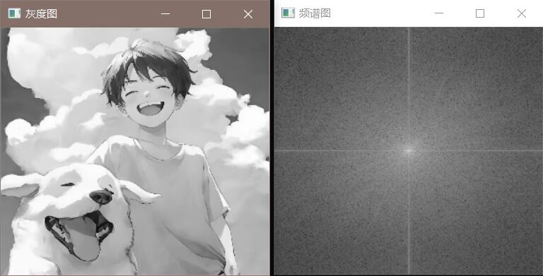
效果展示:
频谱图
频谱图有以下规律:
频谱图从中心点到四周,频率越来越大;
频谱图中心点一般最亮,与原图像平均亮度相关;
频率域滤波就是改变频谱图中高频率或者低频率的值.
频谱图中的点关于中心点对称,对称的两点表示某个频率的波。
两个对称点离中心点的距离代表频率的高低,离中心点越远代表的频率越高。
两个对称点的亮度表示波的幅值,越亮幅值越大。
图像中,低频率代表灰度变化缓慢的信息;高频率代表变化剧烈的信息,如边缘及噪声等。在6中,低频区越亮代表变化缓慢的区域较多,高频区越亮代表图像细节很多。
对称点所在直线的方向为波的方向,与原图中对应的线性信息垂直。如下图,图中有一组平行的线,在频谱图垂直方向也有一条较亮的线(可用于方向滤波,增强或者滤除某个方向的线性特征)。
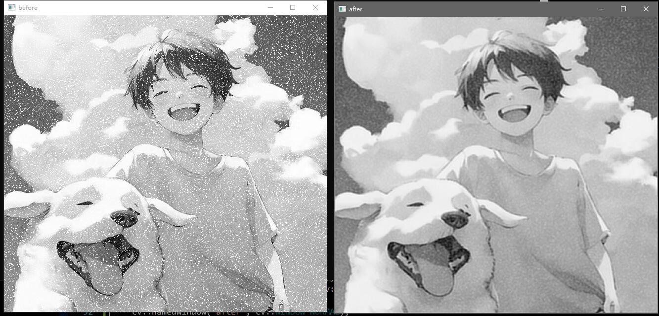
低通滤波
理想低通滤波
通过设置频率半径,半径内的频率大小不变,半径外的频率置为0,保留了低频区,滤除了高频区。
传递函数为:
H ( u , v ) = { 1 , D ( u , v ) ≤ D 0 0 , D ( u , v ) > D 0 H(u,v)=
\begin{cases}
1,\quad D(u,v)\leq D_0\\
0, \quad D(u,v)>D_0
\end{cases}
H ( u , v ) = { 1 , D ( u , v ) ≤ D 0 0 , D ( u , v ) > D 0
其中, D 0 D_0 D 0 D ( u , v ) D(u,v) D ( u , v ) D ( u , v ) = [ ( u − P / 2 ) 2 + ( v − Q / 2 ) 2 ] 1 / 2 D(u,v)=[(u-P/2)^2+(v-Q/2)^2]^{1/2} D ( u , v ) = [ ( u − P / 2 ) 2 + ( v − Q / 2 ) 2 ] 1 / 2
理想低通滤波器由于进行傅里叶变换和傅里叶逆变换时的差异,会导致振铃效应,一般很少使用。
振铃效应:指输出图像的灰度剧烈变化处产生的震荡,就好像钟被敲击后产生的空气震荡
代码:
1 2 3 4 5 6 7 8 9 10 11 12 13 14 15 16 17 18 19 20 21 22 23 24 25 26 27 28 29 30 31 32 33 34 35 36 37 38 39 40 41 42 43 44 45 46 47 48 49 50 51 52 53 54 #include <iostream> #include <opencv2/opencv.hpp> #include "DFT.h" #include "Salt.h" int main () cv::Mat image, output, trf; image = cv::imread ("src/test.jpg" , 0 ); Salt (image, 100000 ); cv::namedWindow ("before" , cv::WINDOW_NORMAL); cv::imshow ("before" , image); DFT (image, output, trf); cv::Mat planes[] = { cv::Mat_ <float >(output), cv::Mat::zeros (output.size (), CV_32F) }; cv::split (trf, planes); cv::Mat trf_real = planes[0 ]; cv::Mat trf_imag = planes[1 ]; int cx = trf_real.rows / 2 ; int cy = trf_real.cols / 2 ; int r = 120 ; for (int i = 0 ; i < trf_real.rows; i ++) for (int j = 0 ; j < trf_real.cols; j ++) if ((i - cx) * (i - cx) + (j - cy) * (j - cy) > r * r) { trf_real.at <float >(i, j) = 0 ; trf_imag.at <float >(i, j) = 0 ; } planes[0 ] = trf_real; planes[1 ] = trf_imag; cv::Mat trf_ilpf; cv::merge (planes, 2 , trf_ilpf); cv::Mat iDft[] = { cv::Mat_ <float >(output), cv::Mat::zeros (output.size (), CV_32F) }; cv::idft (trf_ilpf, trf_ilpf); cv::split (trf_ilpf, iDft); cv::magnitude (iDft[0 ], iDft[1 ], iDft[0 ]); cv::normalize (iDft[0 ], iDft[0 ], 0 , 1 , cv::NORM_MINMAX); cv::namedWindow ("after" , cv::WINDOW_NORMAL); cv::imshow ("after" , iDft[0 ]); cv::waitKey (0 ); return 0 ; }
为了更好的效果,手动添加噪声:
1 2 3 4 5 6 #pragma once #include <opencv2/opencv.hpp> #include <random> void Salt (cv::Mat input, int n) ;
1 2 3 4 5 6 7 8 9 10 11 12 13 14 15 16 17 18 19 #include "Salt.h" void Salt (cv::Mat input, int n) std::default_random_engine generator; std::uniform_int_distribution<int >row (0 , input.rows - 1 ); std::uniform_int_distribution<int >col (0 , input.cols - 1 ); int i, j; for (int k = 0 ; k < n; k ++) { i = row (generator); j = col (generator); if (input.channels () == 1 ) input.at <uchar>(i, j) = 255 ; else if (input.channels () == 3 ) input.at <cv::Vec3b>(i, j) = cv::Vec3b (255 , 255 , 255 ); } }
对图像傅里叶变换:
1 2 3 4 5 6 #pragma once #include <opencv2/opencv.hpp> #include <cmath> void DFT (cv::Mat input, cv::Mat& output, cv::Mat& trf_arr) ;
1 2 3 4 5 6 7 8 9 10 11 12 13 14 15 16 17 18 19 20 21 22 23 24 25 26 27 28 29 30 31 32 33 34 35 36 37 38 39 40 41 42 43 44 45 46 47 48 49 50 51 52 53 54 55 56 57 58 59 60 #include "DFT.h" void DFT (cv::Mat input, cv::Mat& output, cv::Mat& trf_arr) int n = cv::getOptimalDFTSize (input.rows); int m = cv::getOptimalDFTSize (input.cols); cv::copyMakeBorder (input, input, 0 , n - input.rows, 0 , m - input.cols, cv::BORDER_CONSTANT, cv::Scalar::all (0 )); cv::Mat planes[] = { cv::Mat_ <float >(input), cv::Mat::zeros (input.size (), CV_32F) }; cv::merge (planes, 2 , trf_arr); cv::dft (trf_arr, trf_arr); cv::split (trf_arr, planes); cv::Mat trf_img_real = planes[0 ]; cv::Mat trf_img_imag = planes[1 ]; cv::magnitude (planes[0 ], planes[1 ], output); output += cv::Scalar (1 ); log (output, output); cv::normalize (output, output, 0 , 1 , cv::NORM_MINMAX); output = output (cv::Rect (0 , 0 , output.cols & -2 , output.rows & -2 )); int cx = output.cols / 2 , cy = output.rows / 2 ; cv::Mat q0 (output, cv::Rect(0 , 0 , cx, cy)) , q1 (output, cv::Rect(cx, 0 , cx, cy)) ; cv::Mat q2 (output, cv::Rect(0 , cy, cx, cy)) , q3 (output, cv::Rect(cx, cy, cx, cy)) ; cv::Mat tmp; q0. copyTo (tmp); q3. copyTo (q0); tmp.copyTo (q3); q1. copyTo (tmp); q2. copyTo (q1); tmp.copyTo (q2); cv::Mat q00 (trf_img_real, cv::Rect(0 , 0 , cx, cy)) ; cv::Mat q01 (trf_img_real, cv::Rect(cx, 0 , cx, cy)) ; cv::Mat q02 (trf_img_real, cv::Rect(0 , cy, cx, cy)) ; cv::Mat q03 (trf_img_real, cv::Rect(cx, cy, cx, cy)) ; q00. copyTo (tmp); q03. copyTo (q00); tmp.copyTo (q03); q01. copyTo (tmp); q02. copyTo (q01); tmp.copyTo (q02); cv::Mat q10 (trf_img_imag, cv::Rect(0 , 0 , cx, cy)) ; cv::Mat q11 (trf_img_imag, cv::Rect(cx, 0 , cx, cy)) ; cv::Mat q12 (trf_img_imag, cv::Rect(0 , cy, cx, cy)) ; cv::Mat q13 (trf_img_imag, cv::Rect(cx, cy, cx, cy)) ; q10. copyTo (tmp); q13. copyTo (q10); tmp.copyTo (q13); q11. copyTo (tmp); q12. copyTo (q11); tmp.copyTo (q12); planes[0 ] = trf_img_real; planes[1 ] = trf_img_imag; cv::merge (planes, 2 , trf_arr); }
效果展示:
高斯低通滤波
高斯低通滤波器的传递函数为:
H ( u , v ) = e − D 2 ( u , v ) / 2 σ 2 H(u,v)=e^{-D^2(u,v)/2\sigma^2}
H ( u , v ) = e − D 2 ( u , v ) / 2 σ 2
其中, D ( u , v ) D(u,v) D ( u , v ) σ = D 0 \sigma=D_0 σ = D 0
H ( u , v ) = e − D 2 ( u , v ) / 2 D 0 2 H(u,v)=e^{-D^2(u,v)/2D_0^2}
H ( u , v ) = e − D 2 ( u , v ) / 2 D 0 2
那么 D 0 D_0 D 0 D ( u , v ) = D 0 D(u,v)=D_0 D ( u , v ) = D 0
由于高斯函数的傅里叶变换还是高斯函数,所以高斯低通滤波器没有振铃效应。
代码:
DFT.h、DFT.cpp、Salt.h、Salt.cpp同上。
1 2 3 4 5 6 7 8 9 10 11 12 13 14 15 16 17 18 19 20 21 22 23 24 25 26 27 28 29 30 31 32 33 34 35 36 37 38 39 40 41 42 43 44 45 46 47 48 49 50 51 52 53 54 55 #include <iostream> #include <opencv2/opencv.hpp> #include "DFT.h" #include "Salt.h" int main () cv::Mat image, output, trf; image = cv::imread ("src/test.jpg" , 0 ); Salt (image, 100000 ); cv::namedWindow ("before" , cv::WINDOW_NORMAL); cv::imshow ("before" , image); DFT (image, output, trf); cv::Mat planes[] = { cv::Mat_ <float >(output), cv::Mat::zeros (output.size (), CV_32F) }; cv::split (trf, planes); cv::Mat trf_real = planes[0 ]; cv::Mat trf_imag = planes[1 ]; int cx = trf_real.rows / 2 ; int cy = trf_real.cols / 2 ; int r = 80 ; float h; for (int i = 0 ; i < trf_real.rows; i ++) for (int j = 0 ; j < trf_real.cols; j ++) { h = exp (-((i - cx) * (i - cx) + (j - cy) * (j - cy)) / (2.0 * r * r)); trf_real.at <float >(i, j) *= h; trf_imag.at <float >(i, j) *= h; } planes[0 ] = trf_real; planes[1 ] = trf_imag; cv::Mat trf_ilpf; cv::merge (planes, 2 , trf_ilpf); cv::Mat iDft[] = { cv::Mat_ <float >(output), cv::Mat::zeros (output.size (), CV_32F) }; cv::idft (trf_ilpf, trf_ilpf); cv::split (trf_ilpf, iDft); cv::magnitude (iDft[0 ], iDft[1 ], iDft[0 ]); cv::normalize (iDft[0 ], iDft[0 ], 0 , 1 , cv::NORM_MINMAX); cv::namedWindow ("after" , cv::WINDOW_NORMAL); cv::imshow ("after" , iDft[0 ]); cv::waitKey (0 ); return 0 ; }
效果展示:
巴特沃斯低通滤波
巴特沃斯低通滤波器的传递函数为:
H ( u , v ) = 1 1 + [ D ( u , v ) / D 0 ] 2 n H(u,v)=\frac {1} {1+[D(u,v)/D_0]^{2n} }
H ( u , v ) = 1 + [ D ( u , v ) / D 0 ] 2 n 1
其中, D ( u , v ) D(u,v) D ( u , v ) D 0 D_0 D 0 n n n
1阶巴特沃斯滤波器既没有振铃效应也没有负值;2阶巴特沃斯滤波器有轻微振铃效应和较小的负值,但比理想低通滤波器好;高阶巴特沃斯滤波器具有非常明显的振铃效应。2阶和3阶的巴特沃斯滤波器较为合适。
代码:
DFT.h、DFT.cpp、Salt.h、Salt.cpp同上。
1 2 3 4 5 6 7 8 9 10 11 12 13 14 15 16 17 18 19 20 21 22 23 24 25 26 27 28 29 30 31 32 33 34 35 36 37 38 39 40 41 42 43 44 45 46 47 48 49 50 51 52 53 54 55 56 57 58 #include <iostream> #include <opencv2/opencv.hpp> #include "DFT.h" #include "Salt.h" int main () cv::Mat image, output, trf; image = cv::imread ("src/test.jpg" , 0 ); Salt (image, 100000 ); cv::namedWindow ("before" , cv::WINDOW_NORMAL); cv::imshow ("before" , image); DFT (image, output, trf); cv::Mat planes[] = { cv::Mat_ <float >(output), cv::Mat::zeros (output.size (), CV_32F) }; cv::split (trf, planes); cv::Mat trf_real = planes[0 ]; cv::Mat trf_imag = planes[1 ]; int cx = trf_real.rows / 2 ; int cy = trf_real.cols / 2 ; int r = 120 ; float h; float n = 3 ; float d; for (int i = 0 ; i < trf_real.rows; i ++) for (int j = 0 ; j < trf_real.cols; j ++) { d = (i - cx) * (i - cx) + (j - cy) * (j - cy); h = 1.0 / (1 + pow ((d / (r * r)), 2 * n)); trf_real.at <float >(i, j) *= h; trf_imag.at <float >(i, j) *= h; } planes[0 ] = trf_real; planes[1 ] = trf_imag; cv::Mat trf_ilpf; cv::merge (planes, 2 , trf_ilpf); cv::Mat iDft[] = { cv::Mat_ <float >(output), cv::Mat::zeros (output.size (), CV_32F) }; cv::idft (trf_ilpf, trf_ilpf); cv::split (trf_ilpf, iDft); cv::magnitude (iDft[0 ], iDft[1 ], iDft[0 ]); cv::normalize (iDft[0 ], iDft[0 ], 0 , 1 , cv::NORM_MINMAX); cv::namedWindow ("after" , cv::WINDOW_NORMAL); cv::imshow ("after" , iDft[0 ]); cv::waitKey (0 ); return 0 ; }
效果展示:
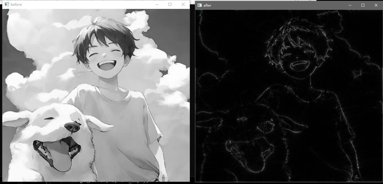
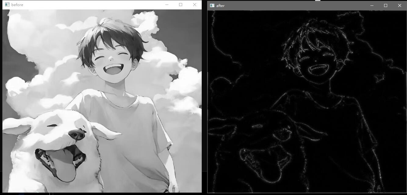
高通滤波
理想高通滤波
通过设置频率半径,半径外的频率大小不变,半径内的频率置为0,保留了高频区,滤除了低频区。
而边缘和其他灰度的急剧变化与高频分量有关,故高通滤波器可以实现边缘锐化。
传递函数为:
H ( u , v ) = { 0 , D ( u , v ) ≤ D 0 1 , D ( u , v ) > D 0 H(u,v)=
\begin{cases}
0,\quad D(u,v)\leq D_0\\
1, \quad D(u,v)>D_0
\end{cases}
H ( u , v ) = { 0 , D ( u , v ) ≤ D 0 1 , D ( u , v ) > D 0
其中, D 0 D_0 D 0 D ( u , v ) D(u,v) D ( u , v ) D ( u , v ) = [ ( u − P / 2 ) 2 + ( v − Q / 2 ) 2 ] 1 / 2 D(u,v)=[(u-P/2)^2+(v-Q/2)^2]^{1/2} D ( u , v ) = [ ( u − P / 2 ) 2 + ( v − Q / 2 ) 2 ] 1 / 2
代码(DFT代码文件见最后):
1 2 3 4 5 6 7 8 9 10 11 12 13 14 15 16 17 18 19 20 21 22 23 24 25 26 27 28 29 30 31 32 33 34 35 36 37 38 39 40 41 42 43 44 45 46 47 48 49 50 51 #include <iostream> #include <opencv2/opencv.hpp> #include "DFT.h" int main () cv::Mat image, output, trf; image = cv::imread ("src/test.jpg" , 0 ); cv::namedWindow ("before" , cv::WINDOW_NORMAL); cv::imshow ("before" , image); DFT (image, output, trf); cv::Mat planes[] = { cv::Mat_ <float >(output), cv::Mat::zeros (output.size (), CV_32F) }; cv::split (trf, planes); cv::Mat trf_real = planes[0 ]; cv::Mat trf_imag = planes[1 ]; int cx = trf_real.rows / 2 ; int cy = trf_real.cols / 2 ; int r = 120 ; for (int i = 0 ; i < trf_real.rows; i ++) for (int j = 0 ; j < trf_real.cols; j ++) if ((i - cx) * (i - cx) + (j - cy) * (j - cy) < r * r) { trf_real.at <float >(i, j) = 0 ; trf_imag.at <float >(i, j) = 0 ; } planes[0 ] = trf_real; planes[1 ] = trf_imag; cv::Mat trf_ilpf; cv::merge (planes, 2 , trf_ilpf); cv::Mat iDft[] = { cv::Mat_ <float >(output), cv::Mat::zeros (output.size (), CV_32F) }; cv::idft (trf_ilpf, trf_ilpf); cv::split (trf_ilpf, iDft); cv::magnitude (iDft[0 ], iDft[1 ], iDft[0 ]); cv::normalize (iDft[0 ], iDft[0 ], 0 , 1 , cv::NORM_MINMAX); cv::namedWindow ("after" , cv::WINDOW_NORMAL); cv::imshow ("after" , iDft[0 ]); cv::waitKey (0 ); return 0 ; }
效果展示:
高斯高通滤波
高斯低通滤波器的传递函数为:
H L P ( u , v ) = e − D 2 ( u , v ) / 2 σ 2 H_{LP}(u,v)=e^{-D^2(u,v)/2\sigma^2}
H L P ( u , v ) = e − D 2 ( u , v ) / 2 σ 2
则高斯高通滤波器传递函数为:
H H P = 1 − H L P ( u , v ) = 1 − e − D 2 ( u , v ) / 2 D 0 2 H_{HP}=1-H_{LP}(u,v)=1-e^{-D^2(u,v)/2D_0^2}
H H P = 1 − H L P ( u , v ) = 1 − e − D 2 ( u , v ) / 2 D 0 2
其中, D ( u , v ) D(u,v) D ( u , v ) D 0 D_0 D 0
代码(DFT代码文件见最后):
1 2 3 4 5 6 7 8 9 10 11 12 13 14 15 16 17 18 19 20 21 22 23 24 25 26 27 28 29 30 31 32 33 34 35 36 37 38 39 40 41 42 43 44 45 46 47 48 49 50 51 52 53 #include <iostream> #include <opencv2/opencv.hpp> #include "DFT.h" int main () cv::Mat image, output, trf; image = cv::imread ("src/test.jpg" , 0 ); cv::namedWindow ("before" , cv::WINDOW_NORMAL); cv::imshow ("before" , image); DFT (image, output, trf); cv::Mat planes[] = { cv::Mat_ <float >(output), cv::Mat::zeros (output.size (), CV_32F) }; cv::split (trf, planes); cv::Mat trf_real = planes[0 ]; cv::Mat trf_imag = planes[1 ]; int cx = trf_real.rows / 2 ; int cy = trf_real.cols / 2 ; int r = 120 ; float h, d; for (int i = 0 ; i < trf_real.rows; i ++) for (int j = 0 ; j < trf_real.cols; j ++) { d = (i - cx) * (i - cx) + (j - cy) * (j - cy); h = 1 - exp (-d / (2.0 * r * r)); trf_real.at <float >(i, j) *= h; trf_imag.at <float >(i, j) *= h; } planes[0 ] = trf_real; planes[1 ] = trf_imag; cv::Mat trf_ilpf; cv::merge (planes, 2 , trf_ilpf); cv::Mat iDft[] = { cv::Mat_ <float >(output), cv::Mat::zeros (output.size (), CV_32F) }; cv::idft (trf_ilpf, trf_ilpf); cv::split (trf_ilpf, iDft); cv::magnitude (iDft[0 ], iDft[1 ], iDft[0 ]); cv::normalize (iDft[0 ], iDft[0 ], 0 , 1 , cv::NORM_MINMAX); cv::namedWindow ("after" , cv::WINDOW_NORMAL); cv::imshow ("after" , iDft[0 ]); cv::waitKey (0 ); return 0 ; }
效果展示:
巴特沃斯高通滤波
巴特沃斯高铁滤波器的传递函数为:
H ( u , v ) = 1 1 + [ D 0 / D ( u , v ) ] 2 n H(u,v)=\frac {1} {1+[D_0/D(u,v)]^{2n} }
H ( u , v ) = 1 + [ D 0 / D ( u , v ) ] 2 n 1
其中, D ( u , v ) D(u,v) D ( u , v ) D 0 D_0 D 0 n n n
代码(DFT代码文件见最后):
1 2 3 4 5 6 7 8 9 10 11 12 13 14 15 16 17 18 19 20 21 22 23 24 25 26 27 28 29 30 31 32 33 34 35 36 37 38 39 40 41 42 43 44 45 46 47 48 49 50 51 52 53 54 #include <iostream> #include <opencv2/opencv.hpp> #include "DFT.h" int main () cv::Mat image, output, trf; image = cv::imread ("src/test.jpg" , 0 ); cv::namedWindow ("before" , cv::WINDOW_NORMAL); cv::imshow ("before" , image); DFT (image, output, trf); cv::Mat planes[] = { cv::Mat_ <float >(output), cv::Mat::zeros (output.size (), CV_32F) }; cv::split (trf, planes); cv::Mat trf_real = planes[0 ]; cv::Mat trf_imag = planes[1 ]; int cx = trf_real.rows / 2 ; int cy = trf_real.cols / 2 ; int r = 120 ; float h, d; float n = 3 ; for (int i = 0 ; i < trf_real.rows; i ++) for (int j = 0 ; j < trf_real.cols; j ++) { d = (i - cx) * (i - cx) + (j - cy) * (j - cy); h = 1.0 / (1 + pow (((r * r) / d), 2 * n)); trf_real.at <float >(i, j) *= h; trf_imag.at <float >(i, j) *= h; } planes[0 ] = trf_real; planes[1 ] = trf_imag; cv::Mat trf_ilpf; cv::merge (planes, 2 , trf_ilpf); cv::Mat iDft[] = { cv::Mat_ <float >(output), cv::Mat::zeros (output.size (), CV_32F) }; cv::idft (trf_ilpf, trf_ilpf); cv::split (trf_ilpf, iDft); cv::magnitude (iDft[0 ], iDft[1 ], iDft[0 ]); cv::normalize (iDft[0 ], iDft[0 ], 0 , 1 , cv::NORM_MINMAX); cv::namedWindow ("after" , cv::WINDOW_NORMAL); cv::imshow ("after" , iDft[0 ]); cv::waitKey (0 ); return 0 ; }
效果展示:
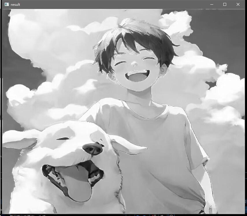
拉普拉斯滤波
频率域中拉普拉斯滤波传递函数为:
H ( u , v ) = − 4 π 2 ( u 2 + v 2 ) = − 4 π 2 [ ( u − P / 2 ) 2 + ( v − Q / 2 ) 2 ] = − 4 π 2 D 2 ( u , v ) H(u,v)=-4\pi^2(u^2+v^2)=-4\pi^2[(u-P/2)^2+(v-Q/2)^2]=-4\pi^2D^2(u,v)
H ( u , v ) = − 4 π 2 ( u 2 + v 2 ) = − 4 π 2 [ ( u − P / 2 ) 2 + ( v − Q / 2 ) 2 ] = − 4 π 2 D 2 ( u , v )
其中, D ( u , v ) D(u,v) D ( u , v )
具体增强实现:
g ( x , y ) = f ( x , y ) + c ∇ 2 f ( x , y ) , ∇ 2 f ( x , y ) = ℑ − 1 [ H ( u , v ) F ( u , v ) ] g(x,y)=f(x,y)+c\nabla^2f(x,y),\nabla^2f(x,y)=\Im^{-1}[H(u,v)F(u,v)]
g ( x , y ) = f ( x , y ) + c ∇ 2 f ( x , y ) , ∇ 2 f ( x , y ) = ℑ − 1 [ H ( u , v ) F ( u , v ) ]
其中, F ( u , v ) F(u,v) F ( u , v ) f ( x , y ) f(x,y) f ( x , y )
代码:
1 2 3 4 5 6 7 8 9 10 11 12 13 14 15 16 17 18 19 20 21 22 23 24 25 26 27 28 29 30 31 32 33 34 35 36 37 38 39 40 41 42 43 44 45 46 47 48 49 50 51 52 53 54 55 56 57 58 59 60 61 62 63 #include <iostream> #include <opencv2/opencv.hpp> #include "DFT.h" int main () cv::Mat image, output, trf; image = cv::imread ("src/test.jpg" , 0 ); cv::namedWindow ("before" , cv::WINDOW_NORMAL); cv::imshow ("before" , image); DFT (image, output, trf); cv::Mat planes[] = { cv::Mat_ <float >(output), cv::Mat::zeros (output.size (), CV_32F) }; cv::split (trf, planes); cv::Mat trf_real = planes[0 ]; cv::Mat trf_imag = planes[1 ]; int cx = trf_real.rows / 2 ; int cy = trf_real.cols / 2 ; float h, d; float pi = 3.1415926 ; for (int i = 0 ; i < trf_real.rows; i ++) for (int j = 0 ; j < trf_real.cols; j ++) { d = (i - cx) * (i - cx) + (j - cy) * (j - cy); h = -4 * pi * pi * d; trf_real.at <float >(i, j) *= h; trf_imag.at <float >(i, j) *= h; } planes[0 ] = trf_real; planes[1 ] = trf_imag; cv::Mat trf_ilpf; cv::merge (planes, 2 , trf_ilpf); cv::Mat iDft[] = { cv::Mat_ <float >(output), cv::Mat::zeros (output.size (), CV_32F) }; cv::idft (trf_ilpf, trf_ilpf); cv::split (trf_ilpf, iDft); cv::magnitude (iDft[0 ], iDft[1 ], iDft[0 ]); cv::normalize (iDft[0 ], iDft[0 ], 0 , 1 , cv::NORM_MINMAX); cv::namedWindow ("after" , cv::WINDOW_NORMAL); cv::imshow ("after" , iDft[0 ]); iDft[0 ].convertTo (iDft[0 ], CV_8U, 255 / 1.0 , 0 ); cv::Mat result (iDft[0 ].size(), CV_8U) ; for (int i = 0 ; i < iDft[0 ].rows; i ++) for (int j = 0 ; j < iDft[0 ].cols; j ++) result.at <uchar>(i, j) = cv::saturate_cast <uchar>(image.at <uchar>(i, j) + iDft[0 ].at <uchar>(i, j)); cv::namedWindow ("result" , cv::WINDOW_NORMAL); cv::imshow ("result" , result); cv::waitKey (0 ); return 0 ; }
效果展示:
高频强调滤波器
还可以设置可调参数,进行调整影响。高频强调滤波的通用公式是:
g ( x , y ) = ℑ − 1 { [ k 1 + k 2 H H P ] F ( u , v ) } g(x,y)=\Im^{-1}\bigg\{\big[k_1+k_2H_{HP}\big]F(u,v)\bigg\}
g ( x , y ) = ℑ − 1 { [ k 1 + k 2 H H P ] F ( u , v ) }
其中, k 1 ≥ 0 k_1\geq0 k 1 ≥ 0 k 2 > 0 k_2>0 k 2 > 0 H H P H_{HP} H H P F ( u , v ) F(u,v) F ( u , v ) f ( u , v ) f(u,v) f ( u , v )
部分代码示例:
1
2
3
4
5
6
7
8
9
for (int i = 0 ; i < trf_real.rows; i ++) for (int j = 0 ; j < trf_real.cols; j ++) { d = (i - cx) * (i - cx) + (j - cy) * (j - cy); h = 0.5 + 0.75 * (1 - exp (-d / (2.0 * r * r))); trf_real.at <float >(i, j) *= h; trf_imag.at <float >(i, j) *= h; }
附DFT代码
1 2 3 4 5 6 #pragma once #include <opencv2/opencv.hpp> #include <cmath> void DFT (cv::Mat input, cv::Mat& output, cv::Mat& trf_arr) ;
1 2 3 4 5 6 7 8 9 10 11 12 13 14 15 16 17 18 19 20 21 22 23 24 25 26 27 28 29 30 31 32 33 34 35 36 37 38 39 40 41 42 43 44 45 46 47 48 49 50 51 52 53 54 55 56 57 58 59 60 #include "DFT.h" void DFT (cv::Mat input, cv::Mat& output, cv::Mat& trf_arr) int n = cv::getOptimalDFTSize (input.rows); int m = cv::getOptimalDFTSize (input.cols); cv::copyMakeBorder (input, input, 0 , n - input.rows, 0 , m - input.cols, cv::BORDER_CONSTANT, cv::Scalar::all (0 )); cv::Mat planes[] = { cv::Mat_ <float >(input), cv::Mat::zeros (input.size (), CV_32F) }; cv::merge (planes, 2 , trf_arr); cv::dft (trf_arr, trf_arr); cv::split (trf_arr, planes); cv::Mat trf_img_real = planes[0 ]; cv::Mat trf_img_imag = planes[1 ]; cv::magnitude (planes[0 ], planes[1 ], output); output += cv::Scalar (1 ); log (output, output); cv::normalize (output, output, 0 , 1 , cv::NORM_MINMAX); output = output (cv::Rect (0 , 0 , output.cols & -2 , output.rows & -2 )); int cx = output.cols / 2 , cy = output.rows / 2 ; cv::Mat q0 (output, cv::Rect(0 , 0 , cx, cy)) , q1 (output, cv::Rect(cx, 0 , cx, cy)) ; cv::Mat q2 (output, cv::Rect(0 , cy, cx, cy)) , q3 (output, cv::Rect(cx, cy, cx, cy)) ; cv::Mat tmp; q0. copyTo (tmp); q3. copyTo (q0); tmp.copyTo (q3); q1. copyTo (tmp); q2. copyTo (q1); tmp.copyTo (q2); cv::Mat q00 (trf_img_real, cv::Rect(0 , 0 , cx, cy)) ; cv::Mat q01 (trf_img_real, cv::Rect(cx, 0 , cx, cy)) ; cv::Mat q02 (trf_img_real, cv::Rect(0 , cy, cx, cy)) ; cv::Mat q03 (trf_img_real, cv::Rect(cx, cy, cx, cy)) ; q00. copyTo (tmp); q03. copyTo (q00); tmp.copyTo (q03); q01. copyTo (tmp); q02. copyTo (q01); tmp.copyTo (q02); cv::Mat q10 (trf_img_imag, cv::Rect(0 , 0 , cx, cy)) ; cv::Mat q11 (trf_img_imag, cv::Rect(cx, 0 , cx, cy)) ; cv::Mat q12 (trf_img_imag, cv::Rect(0 , cy, cx, cy)) ; cv::Mat q13 (trf_img_imag, cv::Rect(cx, cy, cx, cy)) ; q10. copyTo (tmp); q13. copyTo (q10); tmp.copyTo (q13); q11. copyTo (tmp); q12. copyTo (q11); tmp.copyTo (q12); planes[0 ] = trf_img_real; planes[1 ] = trf_img_imag; cv::merge (planes, 2 , trf_arr); }
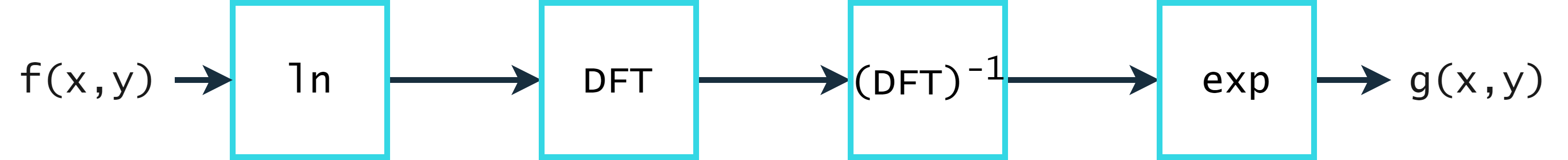
同态滤波
通过一个滤波器传递函数H(u,v),使用不同可控方法影响低频分量和高频分量。
基本原理
图像f(x,y)可以表示为其照射分量i(x,y)和反射分量r(x,y)的乘积。
图像中,认为低频分量与照射分量相联系,高频分量与反射分量相联系。
f ( x , y ) = i ( x , y ) r ( x , y ) f(x,y)=i(x,y)r(x,y)
f ( x , y ) = i ( x , y ) r ( x , y )
乘积的傅里叶变换不是傅里叶变换的乘积。
ℑ [ f ( x , y ) ] ≠ ℑ [ i ( x , y ) ] ℑ [ r ( x , y ) ] \Im [f(x,y)] \neq \Im[i(x,y)]\Im[r(x,y)]
ℑ [ f ( x , y ) ] = ℑ [ i ( x , y ) ] ℑ [ r ( x , y ) ]
故令 z ( x , y ) = ln f ( x , y ) = ln i ( x , y ) + ln r ( x , y ) z(x,y)=\ln f(x,y)=\ln i(x,y)+\ln r(x,y) z ( x , y ) = ln f ( x , y ) = ln i ( x , y ) + ln r ( x , y )
ℑ [ z ( x , y ) ] = ℑ [ ln f ( x , y ) ] = ℑ [ ln i ( x , y ) ] + ℑ [ ln r ( x , y ) ] \Im[z(x,y)]=\Im[\ln f(x,y)]=\Im[\ln i(x,y)]+\Im[\ln r(x,y)]
ℑ [ z ( x , y ) ] = ℑ [ ln f ( x , y ) ] = ℑ [ ln i ( x , y ) ] + ℑ [ ln r ( x , y ) ]
Z ( u , v ) = F i ( u , v ) + F r ( u , v ) Z(u,v)=F_i(u,v)+F_r(u,v)
Z ( u , v ) = F i ( u , v ) + F r ( u , v )
其中, F i ( u , v ) F_i(u,v) F i ( u , v ) F r ( x , y ) F_r(x,y) F r ( x , y ) ln i ( x , y ) \ln i(x,y) ln i ( x , y ) ln r ( x , y ) \ln r(x,y) ln r ( x , y )
使用滤波器传递函数 H ( u , v ) H(u,v) H ( u , v ) Z ( u , v ) Z(u,v) Z ( u , v )
S ( u , v ) = H ( u , v ) Z ( u , v ) = H ( u , v ) F i ( u , v ) + H ( u , v ) F r ( u , v ) S(u,v)=H(u,v)Z(u,v)=H(u,v)F_i(u,v)+H(u,v)F_r(u,v)
S ( u , v ) = H ( u , v ) Z ( u , v ) = H ( u , v ) F i ( u , v ) + H ( u , v ) F r ( u , v )
空间域中滤波后的图像是
s ( x , y ) = ℑ − 1 [ S ( u , v ) ] = ℑ − 1 [ H ( u , v ) F i ( u , v ) ] + ℑ − 1 [ H ( u , v ) F r ( u , v ) ] s(x,y)=\Im^{-1}[S(u,v)]=\Im^{-1}[H(u,v)F_i(u,v)]+\Im^{-1}[H(u,v)F_r(u,v)]
s ( x , y ) = ℑ − 1 [ S ( u , v ) ] = ℑ − 1 [ H ( u , v ) F i ( u , v ) ] + ℑ − 1 [ H ( u , v ) F r ( u , v ) ]
最后通过取滤波后的结果的指数形成输出图像
g ( x , y ) = e s ( x , y ) = e ℑ − 1 [ H ( u , v ) F i ( u , v ) ] e ℑ − 1 [ H ( u , v ) F r ( u , v ) ] g(x,y)=e^{s(x,y)}=e^{\Im^{-1}[H(u,v)F_i(u,v)]}e^{\Im^{-1}[H(u,v)F_r(u,v)]}
g ( x , y ) = e s ( x , y ) = e ℑ − 1 [ H ( u , v ) F i ( u , v ) ] e ℑ − 1 [ H ( u , v ) F r ( u , v ) ]
记
i 0 ( x , y ) = e i ′ ( x , y ) = e ℑ − 1 [ H ( u , v ) F i ( u , v ) ] i_0(x,y)=e^{i'(x,y)}=e^{\Im^{-1}[H(u,v)F_i(u,v)]}
i 0 ( x , y ) = e i ′ ( x , y ) = e ℑ − 1 [ H ( u , v ) F i ( u , v ) ]
为输出图像的照射分量,
记
r 0 ( x , y ) = e r ′ ( x , y ) = e ℑ − 1 [ H ( u , v ) F r ( u , v ) ] r_0(x,y)=e^{r'(x,y)}=e^{\Im^{-1}[H(u,v)F_r(u,v)]}
r 0 ( x , y ) = e r ′ ( x , y ) = e ℑ − 1 [ H ( u , v ) F r ( u , v ) ]
为输出图像的反射分量。
上述滤波方法过程如下图:
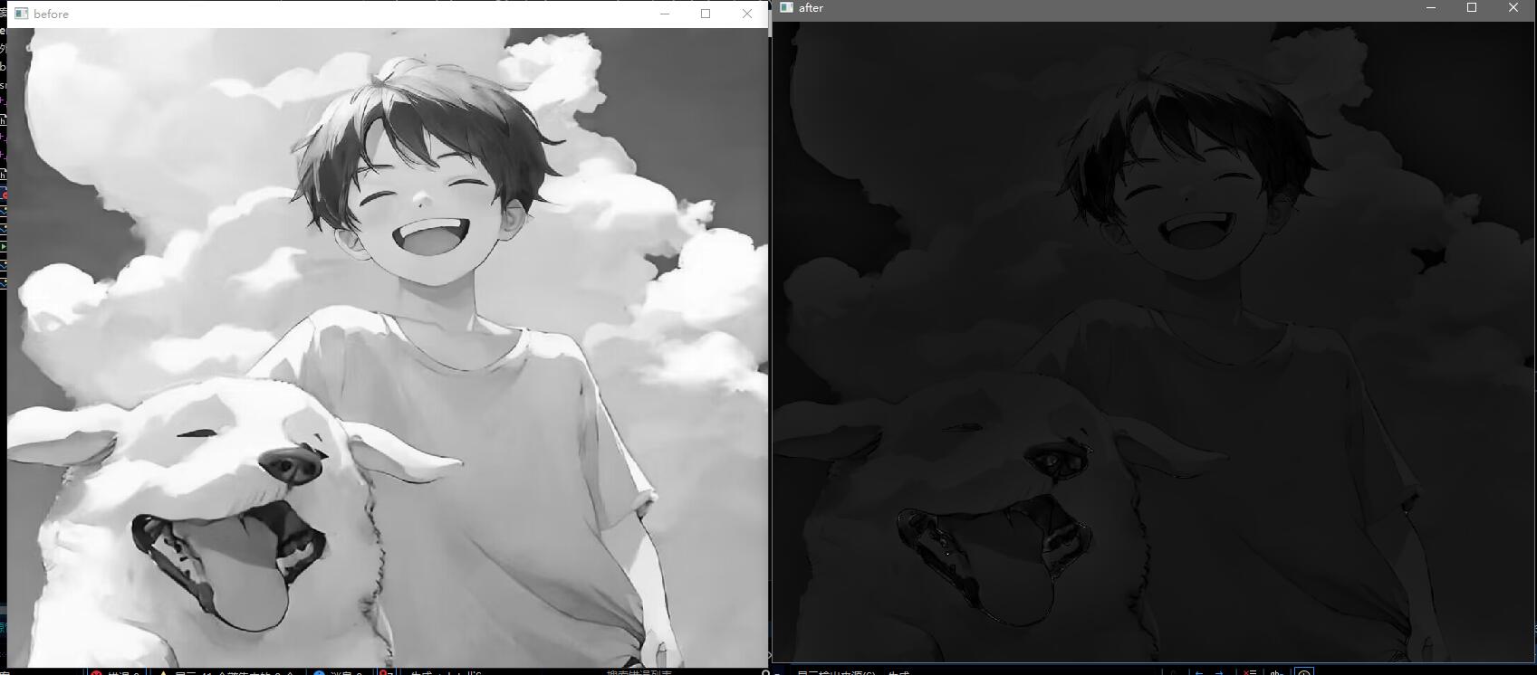
以高斯高通滤波器举例
一般高斯高通滤波器函数:
H ( u , v ) = 1 − e − D 2 ( u , v ) / 2 D 0 2 H(u,v)=1-e^{-D^2(u,v)/2D^2_0}
H ( u , v ) = 1 − e − D 2 ( u , v ) / 2 D 0 2
使用稍微变化的GHPF(Gaussian high-pass filter):
H ( u , v ) = ( γ H − γ L ) [ 1 − e − c D 2 ( u , v ) / D 0 2 ] + γ L H(u,v)=(\gamma_H-\gamma_L)\big[1-e^{-cD^2(u,v)/D_0^2}\big]+\gamma_L
H ( u , v ) = ( γ H − γ L ) [ 1 − e − c D 2 ( u , v ) / D 0 2 ] + γ L
其中,D ( u , v ) D(u,v) D ( u , v ) D 0 D_0 D 0 γ L \gamma_L γ L γ H \gamma_H γ H
变化后的GHPF图像如下:
明显地,减少了低频分量的影响,增加了高频分量的影响。
代码:
1 2 3 4 5 6 7 8 9 10 11 12 13 14 15 16 17 18 19 20 21 22 23 24 25 26 27 28 29 30 31 32 33 34 35 36 37 38 39 40 41 42 43 44 45 46 47 48 49 50 51 52 53 54 55 56 57 58 59 60 61 62 63 64 65 #include <iostream> #include <opencv2/opencv.hpp> #include "DFT.h" int main () cv::Mat image, output, trf; image = cv::imread ("src/test.jpg" , 0 ); cv::namedWindow ("before" , cv::WINDOW_NORMAL); cv::imshow ("before" , image); cv::Mat image_ (image.size(), CV_32F) ; for (int i = 0 ; i < image.rows; i ++) for (int j = 0 ; j < image.cols; j ++) image_.at <float >(i, j) = log (image.at <uchar>(i, j) + 0.1 ); DFT (image_, output, trf); cv::Mat planes[] = { cv::Mat_ <float >(output), cv::Mat::zeros (output.size (), CV_32F) }; cv::split (trf, planes); cv::Mat trf_real = planes[0 ]; cv::Mat trf_imag = planes[1 ]; int cx = trf_real.rows / 2 ; int cy = trf_real.cols / 2 ; int r = 10 ; float h, d; float rh = 3 , rl = 0.5 , c = 5 ; for (int i = 0 ; i < trf_real.rows; i ++) for (int j = 0 ; j < trf_real.cols; j ++) { d = (i - cx) * (i - cx) + (j - cy) * (j - cy); h = (rh - rl) * (1 - exp (-c * d / (r * r))) + rl; trf_real.at <float >(i, j) *= h; trf_imag.at <float >(i, j) *= h; } planes[0 ] = trf_real; planes[1 ] = trf_imag; cv::Mat trf_ilpf; cv::merge (planes, 2 , trf_ilpf); cv::Mat iDft[] = { cv::Mat_ <float >(output), cv::Mat::zeros (output.size (), CV_32F) }; cv::idft (trf_ilpf, trf_ilpf); cv::split (trf_ilpf, iDft); cv::magnitude (iDft[0 ], iDft[1 ], iDft[0 ]); cv::normalize (iDft[0 ], iDft[0 ], 0 , 1 , cv::NORM_MINMAX); cv::exp (iDft[0 ], iDft[0 ]); cv::normalize (iDft[0 ], iDft[0 ], 0 , 1 , cv::NORM_MINMAX); iDft[0 ].convertTo (iDft[0 ], CV_8U, 255 / 1.0 , 0 ); cv::namedWindow ("after" , cv::WINDOW_NORMAL); cv::imshow ("after" , iDft[0 ]); cv::waitKey (0 ); return 0 ; }
效果展示:
1 2 3 4 5 6 #pragma once #include <opencv2/opencv.hpp> #include <cmath> void DFT (cv::Mat input, cv::Mat& output, cv::Mat& trf_arr) ;
1 2 3 4 5 6 7 8 9 10 11 12 13 14 15 16 17 18 19 20 21 22 23 24 25 26 27 28 29 30 31 32 33 34 35 36 37 38 39 40 41 42 43 44 45 46 47 48 49 50 51 52 53 54 55 56 57 58 59 60 #include "DFT.h" void DFT (cv::Mat input, cv::Mat& output, cv::Mat& trf_arr) int n = cv::getOptimalDFTSize (input.rows); int m = cv::getOptimalDFTSize (input.cols); cv::copyMakeBorder (input, input, 0 , n - input.rows, 0 , m - input.cols, cv::BORDER_CONSTANT, cv::Scalar::all (0 )); cv::Mat planes[] = { cv::Mat_ <float >(input), cv::Mat::zeros (input.size (), CV_32F) }; cv::merge (planes, 2 , trf_arr); cv::dft (trf_arr, trf_arr); cv::split (trf_arr, planes); cv::Mat trf_img_real = planes[0 ]; cv::Mat trf_img_imag = planes[1 ]; cv::magnitude (planes[0 ], planes[1 ], output); output += cv::Scalar (1 ); log (output, output); cv::normalize (output, output, 0 , 1 , cv::NORM_MINMAX); output = output (cv::Rect (0 , 0 , output.cols & -2 , output.rows & -2 )); int cx = output.cols / 2 , cy = output.rows / 2 ; cv::Mat q0 (output, cv::Rect(0 , 0 , cx, cy)) , q1 (output, cv::Rect(cx, 0 , cx, cy)) ; cv::Mat q2 (output, cv::Rect(0 , cy, cx, cy)) , q3 (output, cv::Rect(cx, cy, cx, cy)) ; cv::Mat tmp; q0. copyTo (tmp); q3. copyTo (q0); tmp.copyTo (q3); q1. copyTo (tmp); q2. copyTo (q1); tmp.copyTo (q2); cv::Mat q00 (trf_img_real, cv::Rect(0 , 0 , cx, cy)) ; cv::Mat q01 (trf_img_real, cv::Rect(cx, 0 , cx, cy)) ; cv::Mat q02 (trf_img_real, cv::Rect(0 , cy, cx, cy)) ; cv::Mat q03 (trf_img_real, cv::Rect(cx, cy, cx, cy)) ; q00. copyTo (tmp); q03. copyTo (q00); tmp.copyTo (q03); q01. copyTo (tmp); q02. copyTo (q01); tmp.copyTo (q02); cv::Mat q10 (trf_img_imag, cv::Rect(0 , 0 , cx, cy)) ; cv::Mat q11 (trf_img_imag, cv::Rect(cx, 0 , cx, cy)) ; cv::Mat q12 (trf_img_imag, cv::Rect(0 , cy, cx, cy)) ; cv::Mat q13 (trf_img_imag, cv::Rect(cx, cy, cx, cy)) ; q10. copyTo (tmp); q13. copyTo (q10); tmp.copyTo (q13); q11. copyTo (tmp); q12. copyTo (q11); tmp.copyTo (q12); planes[0 ] = trf_img_real; planes[1 ] = trf_img_imag; cv::merge (planes, 2 , trf_arr); }